Neural Computing and Applications · 2025

Efficient time-series approximation
with linear recurrent neural networks

Architecture learning and predictive power

Frieder Stolzenburg1Sandra Litz1Olivia Michael2Oliver Obst2

1 Harz University of Applied Sciences2 Western Sydney University

We study how linear recurrent networks represent time series
and how spectral analysis can reduce their state dimension.

Effect of removing recurrent blocks

Select the two-state blocks to retain. The approximation and errors update for each selection.

A dense recurrence is represented as whole spectral blocks, some of which are omitted to reduce the network.

Enable JavaScript to select blocks and compare errors.

Constructed eight-state example with known dynamics: three sustained oscillations and one decaying oscillation. The dense and block matrices describe the same dynamics in different coordinates. By default, each subset uses an output map fitted by SVD to the first 120 samples only. The retained recurrence and eigenvalues stay fixed during this fit. The later 120 samples measure continuation error. This example isolates block omission and refitting; it does not run reservoir training or automatic model selection. Refitting can redistribute omitted structure across retained blocks, so training and continuation errors are shown separately.

The question

Time-series representation and network dimension

A recurrent network carries a state from one time step to the next. That state can represent oscillations, trends and other temporal structure. A large fitted network may use many more state values than the signal needs. We ask whether that network can be replaced by a smaller recurrence while preserving its approximation of the observations, and how well the reduced recurrence predicts later values.

This paper studies linear recurrent neural networks (LRNNs). Every state update is linear. That makes the dynamics accessible to matrix analysis: we can identify components, measure which ones matter, and construct a smaller recurrence.

x(t + 1) = W x(t)x(t) = Wts

x is the vector of state values, W is the transition matrix, and s is the initial state.

Repeated linear updates can produce nonlinear curves over time, including sinusoids, polynomials and exponentials. The paper concerns these autonomous time series: during prediction, the network evolves without a new external input at every step.

An interactive example

One oscillation, two state values

A pair of state values can rotate around a circle. Reading one of them gives a sinusoid. The point below represents the state values z1 and z2; these values are what rotate.

A two-dimensional state and its sinusoidal output The state moves clockwise around a unit circle. Its first coordinate, shown in blue, is plotted over successive steps on the right. State space z₁z₂ z₁ = 1.00, z₂ = 0.00 read z₁ Output over time 10−1 060 steps

Step 0 / 60

z(t + 1) =cos ωsin ω−sin ωcos ωz(t)

For this block, the eigenvalues are cos ω ± i sin ω. Their angle sets the rotation per step. Scaling the block by a factor ρ makes its radius shrink when ρ < 1, or grow when ρ > 1.

This is an exact, constructed example to explain the representation. It does not train a model in the browser.

The method

Learning and spectral dimension reduction

We first fit an autonomous recurrence using a random linear reservoir and learned output weights. We then construct spectral blocks and evaluate which ones can be omitted within a chosen approximation tolerance.

  1. 01

    Output-weight estimation

    Feed the observed series into a random linear reservoir, a set of extra state values that respond to the observations. Collect its states, then solve a least-squares problem to predict the next observation. Together, the fixed reservoir and learned output weights form the full transition matrix W. This learning step requires no backpropagation through time.

    S(t + 1) ≈ Wout [S(t); R(t)]

    S is the observed series; R holds the reservoir state values.

  2. 02

    Spectral representation of the recurrence

    The spectrum of W gives eigenvalues describing decay, growth and oscillation. Jordan blocks also describe repeated eigenvalues and polynomial factors. A complex conjugate pair is represented together as a real two-state block.

    Ŝ(t) = A Jt y

    J contains the blocks, A reads out the observations, and y is the initial state.

    The Jordan representation motivates the method. The implementation constructs blocks from clustered eigenvalues and refits A to the training trajectory; it does not need an explicit eigenvector basis.

  3. 03

    Block selection by approximation error

    Temporarily omit each whole block, refit the output map, and measure the training error. A large omission error marks an important component. Rank the blocks, then use binary search to find a short ranked prefix within the chosen error tolerance.

    z(t + 1) = Jr z(t)   ·   Ŝ(t) = Ar z(t)

    The retained transition matrix is sparse: its number of recurrent connections grows linearly with its state dimension. The selection searches a fixed ranking, rather than every possible subset of blocks.

See the reduction algorithm
W = fit_next_observation_weights(observations, reservoir)
blocks = real_jordan_blocks(cluster(eigenvalues(W)))

error(kept_blocks):
    J = assemble(kept_blocks)
    Y = rollout(J, fixed_nonzero_start, training_length)
    A = least_squares(Y, observations)
    return RMSE(observations, A @ Y)

rank blocks by error(all_blocks except this_block), largest first
m = binary_search_ranked_prefix(error(prefix) <= tolerance)
return refitted model for blocks[:m]

The Python version additionally audits smaller prefixes because floating-point rank cut-offs can make the measured error non-monotonic. Full details are in the algorithm guide.

Interpolation and extrapolation

Under the stated rank and size assumptions, an LRNN can interpolate a finite sampled time series. That does not guarantee accurate predictions beyond those samples. The eigenvalues, numerical conditioning and structure of the signal matter for extrapolation.

Evidence in the paper

Experiments on structured signals and observed trajectories

The experiments examine both compact representations of structured signals and less regular real-world series.

Multiple superimposed oscillators

Eight-frequency signals with 16-state representations

A signal made from eight sinusoids needs two state values per frequency. The paper reports 16-state LRNNs with error below 10−5 on the fixed MSO signal.

With 150 training samples and at least 70 initial reservoir neurons, the paper reports minimal-size networks in at least 96% of 100 trials. Its random-frequency study also shows difficulties when frequencies are close together or very small.

Paper, Section 5.1
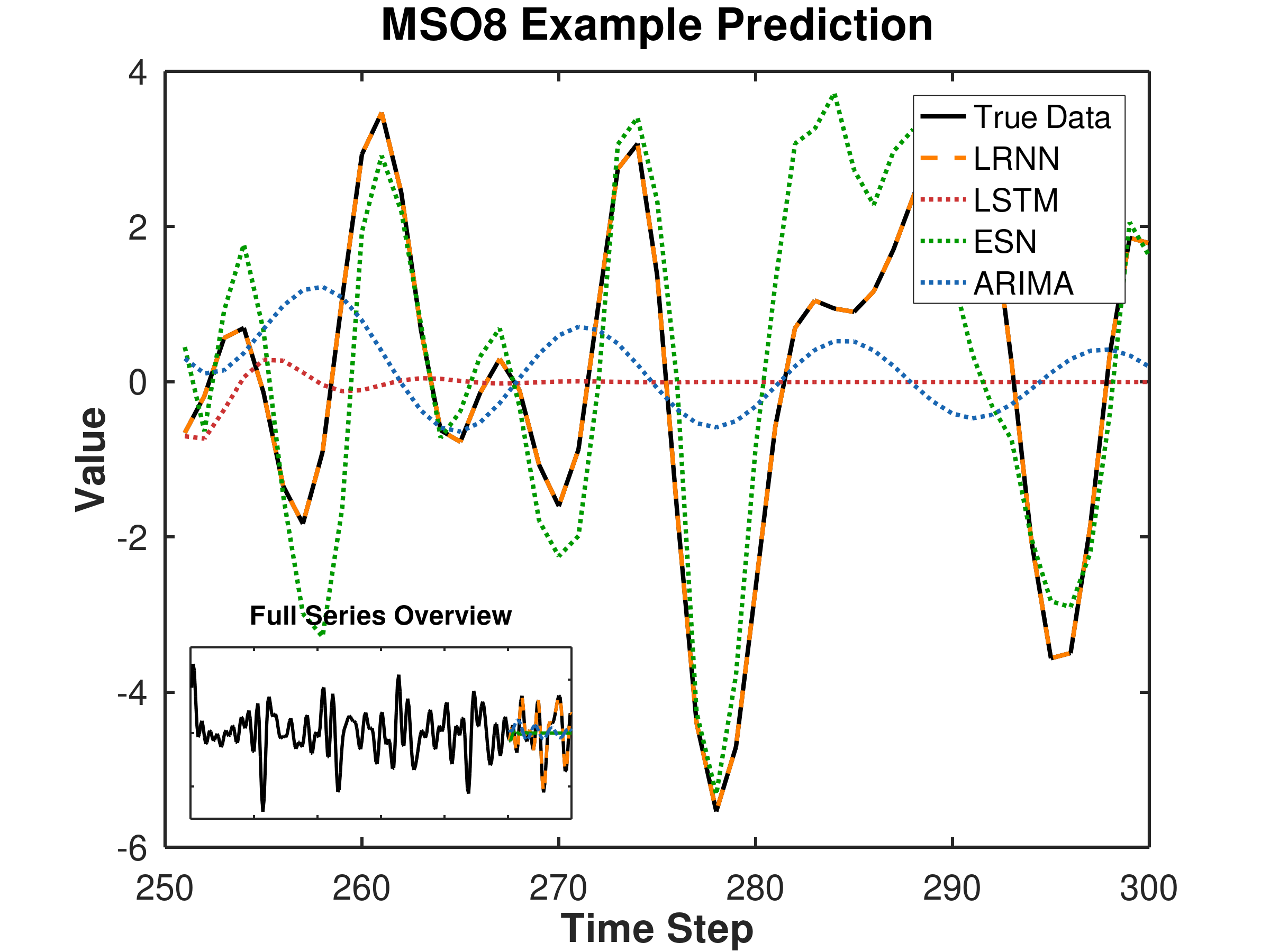
Published MSO comparison: the LRNN follows the eight-frequency signal while the other forecast curves diverge.
MSO forecast comparison. Original figure from the paper’s repository.
Robot soccer simulation

Reconstruction of RoboCup trajectories

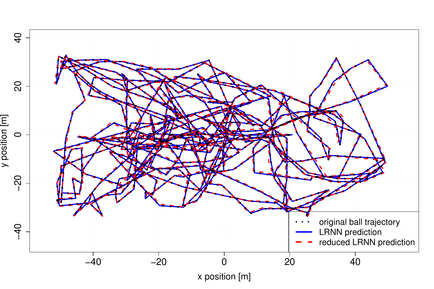
The paper represents a RoboCup 2D game trajectory with an LRNN of 546 neurons, then reduces it to 354 state values while retaining a close approximation of the observed ball path.

This is trajectory reconstruction. The paper also learns from multiple games to examine where a goalkeeper tends to play.

Paper, Section 5.3
Ball trajectory across a RoboCup pitch: the original path, full LRNN reconstruction and reduced LRNN reconstruction are overlaid.
Observed ball trajectory and full/reduced reconstructions. Original repository figure, rendered from PDF.

Number puzzles

Short numerical sequences yield compact recurrences that can be read as formulae. Prediction success depends on the sequence and the information supplied.

Stock prices

LRNNs have the lowest error on 19 of 39 DAX stocks in the paper’s comparison. Across methods, longer forecasts are often little better than carrying forward the last price.

Results above summarise the published paper. The Python results below use separately documented configurations.

Code and reproduction

Implementation and reproducibility

The repository contains the original Octave routines and a self-contained Python library built with NumPy and SciPy. Both use the repository’s BSD 3-Clause licence.

Sinusoid example

The sinusoid example starts with 41 state values, reduces to two, and predicts 100 further samples.

git clone https://github.com/OliverObst/decorating.git
cd decorating/python
uv sync --extra dev --python 3.13
uv run python examples/sinusoid.py

Python 3.11+ is supported. See the installation guide for pip instructions and the API.

Python reproduction

Fitting choices affect forecast accuracy

The default spectrum-and-output-map fit and the optional training-only spectral refinement give different MSO forecast errors. Refinement adjusts the retained eigenvalues and refits the output map, without changing the selected block dimensions or using future observations.

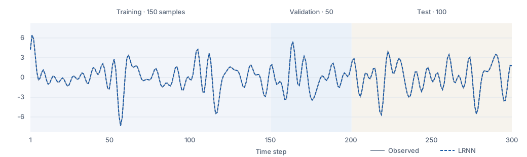
A recorded Python MSO forecast follows the observed signal across training, validation and test segments, using the optional spectral refinement.
Validation-selected Python run, with spectral refinement. 150 training, 50 validation and 100 test samples; 70 initial reservoir units. Curve data come from the verified experiment archive.
Compare all 100-seed Python experiments
Fixed eight-frequency MSO. Seeds 0–99. Validation selects the reported model.
Train / validation / testFittingTest RMSE < 10−5Selected test RMSE
150 / 50 / 100Spectrum + output map0 / 1000.1763
150 / 50 / 100With spectral refinement99 / 1002.061 × 10−14
200 / 50 / 50Spectrum + output map0 / 1002.174 × 10−5
200 / 50 / 50With spectral refinement100 / 1002.726 × 10−14

The shorter configuration uses 70 reservoir units; the longer one uses 198. In the shorter refined condition, one forecast overflows. That failure remains in the denominator. These runs do not reproduce every experiment in the paper or establish every fitting operation used historically.

uv run python experiments/mso.py --profile paper
uv run python experiments/mso.py --profile paper --refine
uv run python experiments/mso.py --profile legacy
uv run python experiments/mso.py --profile legacy --refine

See the accuracy guide and verified experiment records for settings, per-seed results and the Python–Octave comparison.

Reference

Citation

Frieder Stolzenburg, Sandra Litz, Olivia Michael and Oliver Obst.
Neural Computing and Applications 37, 27027–27055 (2025).
doi:10.1007/s00521-025-11655-y

@article{stolzenburg2025lrnn,
  title   = {Efficient time-series approximation with linear recurrent
             neural networks: architecture learning and predictive power},
  author  = {Stolzenburg, Frieder and Litz, Sandra and
             Michael, Olivia and Obst, Oliver},
  journal = {Neural Computing and Applications},
  volume  = {37},
  pages   = {27027--27055},
  year    = {2025},
  doi     = {10.1007/s00521-025-11655-y}
}